Market Update | April 2026
Every month, we share the most important developments in the energy market. We explain how energy prices are determined, highlight trends over several months and years, and provide insight into how the market affects your energy bill.
The Energy Market in April
In April, the energy market was significantly influenced by the rapid growth of solar power. Around noon, this regularly led to low and even negative day-ahead prices, while prices remained high in the morning and evening. The result: a clearduck curvein the daily price trend.
Price differences within a single day reached more than €200/MWh. That is exceptionally high. Batteries, in particular, benefit from these large differences between low and high prices. The value of solar energy was relatively low this month: it stood at just 35% of the average day-ahead price.
We again saw high volatility in the imbalance market, similar to last month. This is partly due to the large share of weather-dependent generation: approximately half of all electricity was produced by solar and wind. In addition, a new record was set (once again): control state 2 was in effect in 46% of the quarter-hours. This makes it more difficult to achieve a consistently positive result through trading on the imbalance market.
1 | Solar Energy
Do you generate solar energy? Then this update is for you. We’ll show you how energy prices in March affected the earnings from solar installations.

April was an exceptionally sunny month. The number of hours of sunshine was significantly higher than normal, meaning that approximately 35% of total electricity generation came from solar panels. During the afternoon hours, when solar energy production was at its peak, electricity prices fell sharply and often dropped below zero. This significantly reduced the value of solar energy. In April, it averaged €29/MWh, just 35% of the average day-ahead price.
1.1 | Volume and value of solar energy
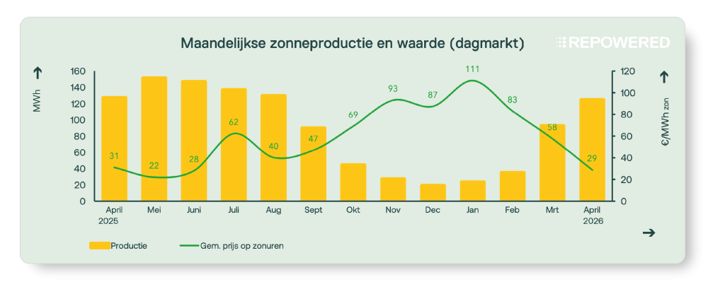
Solar power generation increased significantly compared to previous months. For most of the afternoon, solar power was the primary source of electricity. Due to the high supply, electricity prices fell during these periods.
As shown in the chart above, solar panel owners received an average of €29/MWh for the energy they generated, just 35% of the average day-ahead price of €85/MWh.
1.2 | Negative prices on the spot market
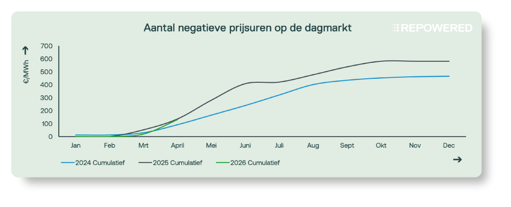
There were a relatively large number of instances of negative prices on the day-ahead market in April. In total, there were 112 hours with negative prices. On nearly two-thirds of all days, the price fell below zero. In addition, 59 of these hours fell within consecutive six-hour blocks, resulting in solar farms with an SDE++ subsidy granted after 2016 receiving a lower subsidy.
Not only were prices often negative, but they were also significantly lower than average. On several occasions, prices fell below −100 €/MWh. On April 26, afternoon prices even dropped to nearly −500 €/MWh. This means that some market participants were willing to pay more than €500/MWh just to continue generating power.
This underscores once again that there is insufficient flexibility in the current energy system. A great deal of renewable energy is being generated, but there are too few entities capable of using this electricity during sunny periods.
2 | Batteries
Do you have a battery? Then this update is for you. We’ll show you how energy prices in March affected the earning potential of batteries.

The revenue potential for batteries in April was comparable to that in March and significantly better than during the winter months. Very low midday prices, driven by high solar generation, and expensive evening hours created strong day-ahead arbitrage opportunities, allowing batteries to charge when prices are low and discharge when prices are high.
In addition, the increasing production of solar and wind energy led to greater volatility in the imbalance market. At the same time, a large proportion of the quarters —46%—ended in control state 2 . This significantly limited the earning potential in the imbalance market.
2.1 | Day Market: Price Distribution
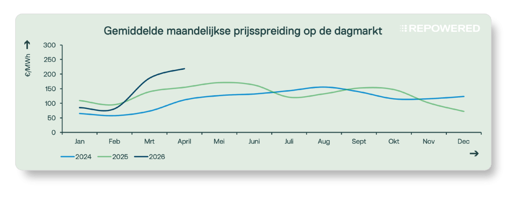
The profit potential on the day-ahead market was once again high last month. This was mainly driven by a sharp contrast between very low prices during sunny afternoon hours and high prices in the morning and evening, caused by higher gas prices. Batteries were able to capitalize on this by storing excess solar energy and discharging it during the expensive evening hours. The average daily price spread rose to €218/MWh, the highest difference to date.
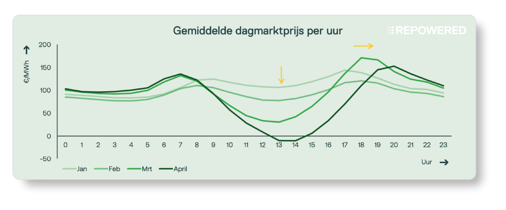
When intraday price fluctuations are driven by low midday prices and high prices in the morning and evening, this creates what is known as a duck curve (a duck-like pattern). As we move into spring, afternoon prices on the day-ahead market continue to fall due to the increase in solar energy. Meanwhile, prices in the morning and evening remain relatively stable, as they are primarily determined by gas-fired power plants.
Another notable feature of the curve is a horizontal shift, with the evening peak occurring later. This is due to the fact that daylight hours are longer and the transition from standard time to daylight saving time, which means that solar panels continue to generate electricity until later in the afternoon.
2.2 | Imbalance Market: Price Dispersion

In April, prices on the imbalance market were largely comparable to those in March and, once again, more volatile than in the previous four to five months. This can be partly explained by the high share of solar and wind energy in the electricity mix—approximately 50%. These weather-dependent energy sources are difficult to predict a day in advance. When actual production deviates from the forecast and from what was offered on the day-ahead market, an imbalance arises. Consequently, a higher share of solar and wind energy generally increases volatility on the imbalance market.
In addition, a higher volume of renewable energy generation often leads to higher imbalance prices. This is due to the startup costs of gas-fired power plants. Because these plants operate less frequently when renewable energy production is high, they sometimes need to be started up to provide balancing energy when TenneT requests it. They charge higher fees for this, which is reflected in the price on the imbalance market.
Together, these two factors are causing an increase in volatility in the imbalance market. The average price differences amounted to €808/MWh.
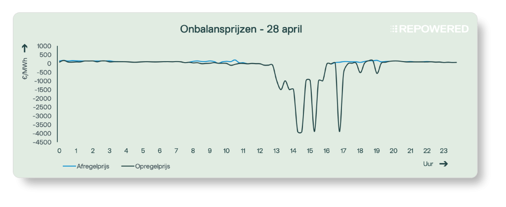
Unlike in recent months, there were virtually no extreme price spikes this month. The only exceptional spike occurred on April 28 and went in an unusual direction—namely, downward. This extremely negative price meant that market participants who produced too much or purchased too little faced imbalance charges of approximately €4,000/MWh. Producing less or purchasing more, on the other hand, was rewarded.
2.3 | Imbalance Market: Control State 2
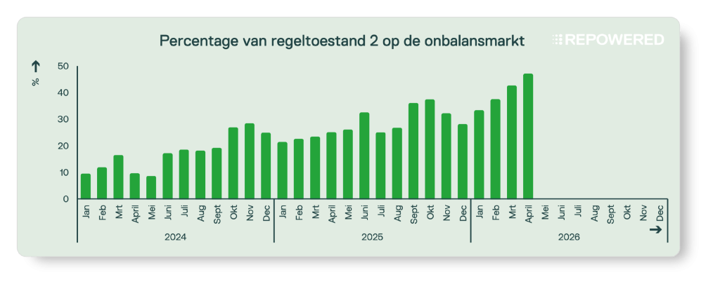
The percentage of quarters that ended in status 2 reached a new record high of 46% this month . This is exceptionally high.
The explanation for the persistently high number of quarters in control state 2 has changed over time. Initially, the increase was mainly attributed to the variability of wind energy. Wind energy production is difficult to predict and can change rapidly due to shifts in wind speed and direction. Later, it was mainly explained by the emergence of so-called passive balancing, in which parties adjust to the imbalance on the power grid based on the balance delta published by TenneT. Recently, it has increasingly been linked to the European integration of energy markets, such as PICASSO.
Despite TenneT’s ongoing efforts to improve the balancing mechanisms, it has not yet been possible to achieve a sustained reduction in the number of quarter-hours in control state 2.
Feeling lost in technical jargon?
Don't worry! We've got a handy glossary ready for you👇